Python GPU Programming with Numba and CuPy

In a previous blog, we looked at using Numba to speed up Python code by using a just-in-time (JIT) compiler and multiple cores. The speed-up is remarkable with small changes to the existing code.

In this blog post, we will continue exploring the Numba ecosystem and implement the Gauss map on the GPU, gaining further speed up while still writing Python code. We will also look at CuPy which is another way to write and run GPU code. Instead of being Pythonic, it allows hybrid programming where the GPU code is written in CUDA but executed in Python.

One key advantage of hybrid programming is writing software in your preferred language while optimising performance-critical sections in a faster language - the best of both worlds!

We won't provide a detailed beginners tutorial but instead, a commentary on how we went from CPU code to GPU code. We will also give benchmarks to see how much of a speed-up we get from using the GPU. This at least gives an idea of whether your research problem is suited for a GPU and the difficulty of implementing GPU code.

Before discussing how to program a GPU, it is important to recap the architecture of a computer and a GPU.

GPU Architecture

So far, we have been running code exclusively on a CPU, which has multiple cores. For example, the ddy nodes have 48 cores each. Each of these cores can run one or more threads, either independently or as part of a larger task. Depending on the workload, these threads may execute different instructions and complete at different times. To leverage multiple cores for parallel execution in Python, you can use libraries like multiprocessing.

Overthreading

Your CPU code should only execute one thread per core on Apocrita. Otherwise, it will lead to overthreading and node alarms, impacting your and others' jobs.

For more tips, see this blog post.

A GPU, however, has thousands of CUDA cores, this is illustrated in Figure 1. Each CUDA core is able to execute instructions all in parallel, enabling fast parallel computation.

Figure 1: A simplified diagram of cores in a CPU and a GPU. Typically a CPU can have about 4 to 32 cores in commercial-grade CPUs or more in HPC systems. Whereas a GPU has thousands of CUDA cores.

However, there are a few weaknesses with GPUs which must be considered when deciding if using a GPU is best for your code.

Memory Limitations

The photo in Figure 2 shows a V100 graphics card, which houses the GPU and VRAM. As discussed previously, the GPU is the main processing unit with thousands of CUDA cores. VRAM is dedicated memory for the GPU to access via a high-speed bus. This card is typically installed in a PCIe slot, as shown in Figures 2 and 3. Commonly, the CPU and RAM together are called the host and the GPU and VRAM together are called the device.

Figure 2: A photograph of a V100 card slotted in a PCIe slot. This PCIe slot is part of a raiser cable which connects the card to a motherboard.

Figure 3: A diagram showing a graphics card, which houses the GPU and VRAM, connected to the motherboard via PCIe. The motherboard also houses the CPU and RAM. The CPU and RAM transfer data between each other via fast internal buses and similarly between the GPU and VRAM.

As a programmer, you are responsible for allocating memory for the host, but also for the device. In programming languages, such as Python, host memory allocation is dynamic and easier compared with older languages such as C. However, as we see later, it is important to keep track in your code if a piece of memory is located in RAM or VRAM so that the CPU and GPU can work with data in their respective dedicated memory.

Avoid Too Many Transfers

The programmer is also responsible for transferring data between the host and the device over the PCIe bus in their code. It should be noted that the transfer speed is slower compared with the internal buses, which can lead to potential bottlenecks if data is transferred back and forth too often.

Avoid too many host-to-device and device-to-host transfers.

Manage and Plan Memory Resources

It should also be noted that for most computers, typically, VRAM is smaller than RAM. For example, our H100 and A100 GPUs can have VRAM of 80 GB. However, exclusive use of a ddy node allows access to more than 300 GB of RAM. Thus it is important to plan how much data you want to store in VRAM. If you find your data or model cannot all fit in VRAM, consider if your problem or data can be split into batches.

Warps and Threads

When programming a GPU, groups of 32 threads are organised in warps. Threads in a warp can only execute one instruction at a time. However, control flows, such as if statements, can be a problem because they introduce branch divergence. This is where some threads want to execute one branch of the if statement, and the other threads want to work on the other branch. When this happens in a warp, each branch is executed serially. This wastes GPU resources because some threads are stalled when either branch is executed. This is illustrated in Figure 4.

As a result, pleasingly parallel tasks are more suited to GPUs. In contrast, problems with lots of complex conditionals and boundaries may struggle to make the most of a GPU.

Figure 4: The left shows the pseudo-code of an if statement. The right shows threads in a warp. For illustration purposes, 8 threads in a warp are shown as arrows. Each branch of the if statement is executed serially, causing a branch divergence. Threads in one branch execute their commands first before threads in the other branch can.

Limited Precision

GPUs are optimized for 32-bit numbers which allow for much faster computations than 64-bit numbers. While numerical precision may be lost with 32-bit arithmetic, it often provides a significant speed-up.

GPU Development Tips

When writing code for a GPU, I recommend implementing a CPU version first followed by the GPU version. These two version can be compared for the following:

• Correctness: The CPU and GPU versions should produce the same results. If they don't, then there must be an error in one of your implementations or the limitations of the GPU are having an effect.
• Benchmarks: You can benchmark the CPU and GPU versions to see which one runs faster. If you find your GPU version is slower, your problem may not be suited for a GPU or there are bottlenecks in your GPU code.

The Gauss Map

The implementations of the Gauss map will follow from a previous blog post. To quickly recap, the Gauss map is a chaotic attractor described by the recurrence relation:

\[ \Large{x_{n+1} = e^{-\alpha x_{n}^{2}} + \beta } \]

To produce bifurcation diagrams, we:

1. Choose a value of \(\alpha\).
2. Scan \(\beta\) from a minimum to a maximum value along the x-axis.
3. For each \(\beta\), initialise \(x_{0}\) to 0.
4. Iterate the recurrence relation a few times to get rid of transients.
5. Iterate again, plotting the intensity of the histogram of the values as a column of points.

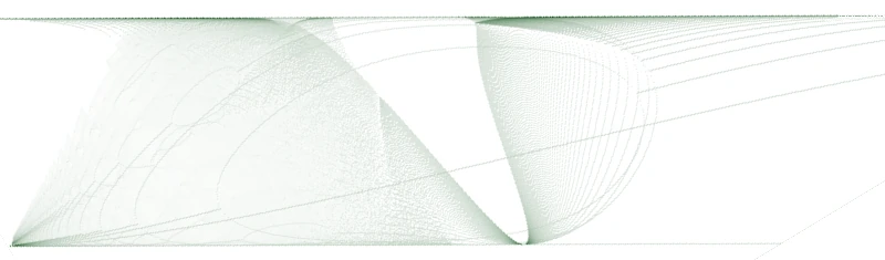
To push the GPU to work hard, we'll extend the problem by scanning \(\alpha\) over a range of values, producing an array of bifurcation diagrams. By putting the diagrams together, we can produce a video as shown in Figure 5. This can be done by saving the diagrams as a sequence of images, using, for example, Pillow PIL, and stitching the images together using ffmpeg or other similar software.

Figure 5: Bifurcation diagrams of the Gauss map. Each column represents a different value of \(\beta\) varying from -1 to 1. Each frame represents a different value of \(\alpha\) varying from 1 to 20.

We could implement the Gauss map such that each thread on a GPU can work on a \((\alpha, \beta)\) pair. The problem is also pleasingly parallel without any branch divergence as each thread iterates through the recurrence relation and keep track of values for the histogram without any conditions.

CPU Numba Implementation

The code for our CPU implementation is shown below at the end of this subsection. Our focus is on the computation for the bifurcation diagram so our benchmark timings target that.

We've used numba to speed up our code. This is done by using @njit(parallel=True) along with for i_alpha in prange(len(alpha))so that each core is working on a value of \(\alpha\), producing values for a bifurcation diagram. This is illustrated in Figure 6. Relevant functions are decorated with @njit so that the parallelised code is compiled with a JIT compiler when running the code, making it usable and faster when compiled.

Figure 6: An animation of 4 cores being assigned to work on a value of \(\alpha\) each. The cores work independently and may finish at different times. Once finished, they move on to the next value of \(\alpha\) to work on.

Compared with the previous blog, we increased the parameters to push the CPU, and later on the GPU, to work hard. For example, we are making diagrams of size 1920 × 1080, iterating through the recurrence relation a million times and producing 1000 diagrams with different values of \(\alpha\). A million evaluations of the recurrence relation are excessive for plotting purposes, but chosen to stress the CPU and GPU when we benchmark them later on.

We've also used 32-bit numbers by enforcing np.float32 and np.int32 types when declaring numpy arrays. The purpose of this is to try and have a fair comparison of benchmarks when comparing it to the GPU version, which is optimised for 32-bit numbers.

Lastly, we've avoided the use of np.histogram(), unlike in the previous blog. This is because when we go to use numba.cuda to implement the GPU version of the Gauss map, a lot of numpy functions become unavailable. As a result, we adjust our implementation of the Gauss map to avoid using numpy and check it still reproduces the same results.

Benchmarks - CPU

We ran our CPU implementation on the ddy nodes with different numbers of cores. Figure 7 shows the resulting benchmarks. Doubling the number of CPU cores results in a corresponding doubling of the CPU implementation's speed. This indicates that the CPU cores remain well-utilised throughout execution, with minimal overhead from managing multiple threads. Such efficient utilisation suggests that the algorithm, if pleasingly parallel, may be well-suited for a GPU implementation.

Sizing your jobs

For this particular code, we've shown that requesting and using more CPU cores will improve performance. However on Apocrita, requesting more cores may result in longer queueing times.

Balance your resource requests for your job.

See this blog post for more tips.

Figure 7: Benchmarks from running our CPU implementation on a ddy node with different numbers of CPU cores.

gauss-cpu.py

from numba import njit, prange
import numpy as np
from PIL import Image

import math
import os
import time


OUTPUT_PATH = "cpu"


@njit
def gauss_map(x, alpha, beta):
    return math.exp(-alpha * x**2) + beta


@njit
def gauss_scan(alpha, beta, image, i_alpha, n_points, bin_start, bin_end, skip):

    n_bin = image.shape[2]
    bin_width = (bin_end - bin_start) / n_bin
    count = np.zeros(n_bin, np.int32)

    for i_beta, beta_i in enumerate(beta):

        count[:] = 0
        x = 0.0
        for _ in range(skip):
            x = gauss_map(x, alpha, beta_i)

        for _ in range(n_points):
            x = gauss_map(x, alpha, beta_i)

            x_bin = int(math.floor((x - bin_start) / bin_width))

            if x_bin >= 0 and x_bin < n_bin:
                count[x_bin] += 1

        image[i_alpha, i_beta, :] = (
                1 - np.sqrt(count.astype(np.float32) / float(n_points)))


@njit(parallel=True)
def gauss_image(alpha, beta_min=-1.0, beta_max=1.0, width=1920, height=1080,
                bin_start=-1.0, bin_end=1.5, skip=200, n_points=1_000_000):

    image = np.zeros((alpha.shape[0], width, height), np.float32)
    beta = np.linspace(beta_min, beta_max, width).astype(np.float32)
    for i_alpha in prange(len(alpha)):
        gauss_scan(alpha[i_alpha], beta, image, i_alpha, n_points, bin_start,
                   bin_end, skip)
    return image


def main():
    time_start = time.perf_counter()
    alpha = np.linspace(0, 100, 1000, dtype=np.float32)
    image_array = gauss_image(alpha)
    print(f"Time: {time.perf_counter() - time_start} s")
    print("Saving images...")
    if not os.path.exists(OUTPUT_PATH):
        os.makedirs(OUTPUT_PATH)
    for i in range(len(alpha)):
        image = Image.fromarray((255 * image_array[i, :, :].T).astype(np.uint8))
        image.save(os.path.join(OUTPUT_PATH, f"cpu{i}.png"))


if __name__ == "__main__":
    main()

GPU Numba Implementation

We now move on to the GPU implementation using numba.cuda, the code is shown below at the end of this subsection.

Functions to be run on the device are decorated with @cuda.jit. In our implementation, those functions are gauss_slice() and gauss_map(). The function gauss_slice() is called a kernel function. This is a function which runs on the device but is called from the host, verified by noticing that gauss_slice() is called from the non-decorated function gauss_image(). The kernel function is launched and executed for each requested thread on the GPU. The function gauss_map() is a device function, this is a function which runs on the device and is called from the device. This can be seen in our implementation as gauss_map() is called from gauss_slice(). This distinction is important later on.

In our problem and implementation, we would like each thread to do calculations for a unique \((\alpha, \beta)\) pair. Each thread is given a unique pair of indices, using idx, idy = cuda.grid(2), which can be used to assign a unique \((\alpha, \beta)\) pair.

We first have to organise our threads into blocks by specifying the block dimension. In our code, we've used a block dimension of 16 × 2. This means each block has 32 threads, each thread working on a unique \((\alpha, \beta)\) pair from 16 values of \(\beta\) and 2 values of \(\alpha\).

Given the block dimension, we specify the number of blocks in each dimension to ensure we have a sufficient number of threads for our problem. Figure 8 illustrates how blocks are allocated to cover all unique pairs of \((\alpha, \beta)\) we want to compute for. The code snippet below shows how the number blocks are calculated.

block_dim_x = 16
block_dim_y = 2
n_block_x = math.ceil(width / block_dim_x)
n_block_y = math.ceil(alpha_h.shape[0] / block_dim_y)

The block dimension and the number of blocks together is known as the grid configuration. The block dimension is hard-coded in our implementation but can be generalised to be a user-specified parameter.

Advice for Selecting the Block Dimension

It is usually advised that the number of threads in a block is a multiple of 32. This is because the 32 threads in a warp run in parallel on a GPU. It is possible that certain grid configurations are more optimal than others but this is beyond the scope of this blog.

Because the number of values of \(\alpha\) and \(\beta\) we want to investigate may not be exactly divisible by the block dimensions, there may be more threads than needed. This is illustrated in Figure 8. To ensure those excessive threads do not do any work and to prevent out-of-bounds memory access, we do a boundary check with

if idx >= beta.shape[0]:
    return
if idy >= alpha.shape[0]:
    return

Figure 8: Blocks, of dimensions 16 × 2, are allocated unique pairs of \((\alpha, \beta)\). The hatched areas represent values of \((\alpha, \beta)\) to be computed. The different colours represent different blocks. Some blocks may extend beyond the hatched area, hence a boundary check should be done to ensure excessive threads do not do any work and to prevent out-of-bounds memory access.

We now discuss memory management, which mostly happens in the function gauss_image(). Arrays created using numpy are on the host. There are a few ways to allocate arrays on the device, known as device arrays. An empty device array can be allocated using cuda.device_array(). There's also an option to transfer host data to the device, this can be done by passing a numpy array to the function cuda.to_device() which then returns a device array. Device arrays, along with the grid configuration, are passed to the kernel function for it to be processed by the GPU.

Any temporary arrays required by the device will need to be preallocated. For example, we've allocated an empty array, called count_d, which stores the histogram counts for each \((\alpha, \beta)\) pair on the device.

To call the kernel function, we provide the grid configuration in square brackets and then the arguments in regular brackets. The code snippet below shows this.

gauss_slice[
    (n_block_x, n_block_y), (block_dim_x, block_dim_y)](
    alpha_d, beta_d, count_d, img_d, n_points, bin_start, bin_end, skip)

Once the calculations are done, we use the method copy_to_host() to transfer the results from the device to the host. As a convention for naming variables and as an aid, we use the suffixes _h and _d to indicate a variable on RAM and VRAM respectively. They stand for host and device respectively.

As discussed in the previous section, some numpy functions are unavailable inside @cuda.jit decorated functions, such as np.histogram(). These unavailable functions may need to be reimplemented using the math library, which has more available functions. Fortunately, the histogram counting for the Gauss map is fairly straightforward to implement using only the math library.

Benchmarks - GPU with numba

We ran benchmarks for our CPU and GPU numba.cuda implementations of the Gauss map. For the GPU implementation, we've used the V100, A100 and H100 GPUs. Below are the nodes used for the benchmarks

• CPU: ddy node with all 48 cores exclusively
• V100: sbg node
• A100: sbg node
• H100: xdg node

The benchmarks are shown in Figure 9.

Figure 9: Benchmarks of the Gauss map using CPU on addy and the V100, A100 and H100 GPUs.

Compared with the CPU version, the GPU implementations running on the newer A100 and H100 GPUs have a speed-up of about 17× and 29× respectively. This is remarkable despite the CPU version using all cores on a ddy node. This is a good result to see and paid off the effort of implementing the GPU version. For this problem, using a GPU is far more beneficial than requesting more CPU cores.

We've also found it unusual the benchmarks for the V100 only show about a 1.9× speed up compared with the CPU version. In such a scenario, we may have to play about with the grid configuration to improve performance or are better off requesting and using the newer A100 and H100 GPUs which have a significant speed-up. We will explore grid configurations in a future blog entry.

gauss-numba-cuda.py

from numba import cuda
import numpy as np
from PIL import Image

import math
import os
import time


OUTPUT_PATH = "numba-cuda"


@cuda.jit
def gauss_map(x, alpha, beta):
    return math.exp(-alpha * x**2) + beta


@cuda.jit
def gauss_slice(alpha, beta, count, image, n_points, bin_start, bin_end, skip):

    idx, idy = cuda.grid(2)
    if idx >= beta.shape[0]:
        return
    if idy >= alpha.shape[0]:
        return

    n_bin = image.shape[1]
    bin_width = (bin_end - bin_start) / n_bin
    alpha = alpha[idy]
    beta = beta[idx]

    x = 0.0
    for _ in range(skip):
        x = gauss_map(x, alpha, beta)

    for _ in range(n_points):
        x = gauss_map(x, alpha, beta)

        x_bin = int(math.floor((x - bin_start) / bin_width))

        if x_bin >= 0 and x_bin < n_bin:
            count[idy, x_bin, idx] += 1

    for x_bin in range(n_bin):
        image[idy, x_bin, idx] = (
            1 - math.sqrt(float(count[idy, x_bin, idx]) / float(n_points)))


def gauss_image(alpha_h, beta_min=-1.0, beta_max=1.0, width=1920, height=1080,
                bin_start=-1.0, bin_end=1.5, skip=200, n_points=1_000_000):

    beta_h = np.linspace(beta_min, beta_max, width, dtype=np.float32)

    alpha_d = cuda.to_device(alpha_h)
    beta_d = cuda.to_device(beta_h)

    img_d = cuda.device_array((alpha_h.shape[0], height, width), np.float32)
    count_d = cuda.device_array((alpha_h.shape[0], height, width), np.int32)

    block_dim_x = 16
    block_dim_y = 2
    n_block_x = math.ceil(width / block_dim_x)
    n_block_y = math.ceil(alpha_h.shape[0] / block_dim_y)

    gauss_slice[
        (n_block_x, n_block_y), (block_dim_x, block_dim_y)](
        alpha_d, beta_d, count_d, img_d, n_points, bin_start, bin_end, skip)

    img_h = img_d.copy_to_host()

    return img_h


def main():
    time_start = time.perf_counter()
    alpha = np.linspace(0, 100, 1000, dtype=np.float32)
    image_array = gauss_image(alpha)
    print(f"Time: {time.perf_counter() - time_start} s")
    print("Saving images...")
    if not os.path.exists(OUTPUT_PATH):
        os.makedirs(OUTPUT_PATH)
    for i in range(len(alpha)):
        image = Image.fromarray((255 * image_array[i, :, :]).astype(np.uint8))
        image.save(os.path.join(OUTPUT_PATH, f"gpu{i}.png"))


if __name__ == "__main__":
    main()

GPU CuPy Implementation

Another way to program and run GPU code in Python is to do hybrid programming with CuPy. We write CPU code in Python and GPU code in CUDA. The CUDA code can be called from Python. This has the advantage that the programmer can work closer to bare metal and the code becomes more general. For example, the same CUDA code can be run in MATLAB, or in Java using JCuda. In another scenario, you may come across existing CUDA code you want to run in Python. The main disadvantage is that coding in CUDA is more difficult, requiring C-like expertise.

Both Python CPU and CUDA GPU code are shown below at the end of this subsection.

Looking at the Python code at a glance, this is similar to using numba.cuda because the library cupy offers the same mechanics as numba.cuda. For example, cupy.zeros() to allocate a device array, cupy.asarray() to copy data from the host to the device and .get() to copy data from the device to the host.

The GPU code is in a different language called CUDA which is more similar to C than Python. A tutorial on the CUDA language is beyond the scope of this blog but we'll make a few brief points. The first point is that, like C, the language is statically typed. This means every variable must have its types declared. Another point is that the kernel function and device function are distinguished using the keywords extern "C" __global__ and __device__ respectively. Lastly, pointers are passed to the kernel function, rather than device arrays when using numba.cuda. A pointer contains the address to a piece of data in memory which can be de-referenced to obtain the value of the data. You can also do pointer arithmetic, such as addition, to access sequential data in an array.

To bridge the gap between the Python and CUDA code, we first compile the .cu source code into a .ptx file. This is done using the nvcc compiler. The bash command below shows how to compile for the A100 GPU.

nvcc -ptx gauss.cu -o gauss.ptx -arch=sm_80

The nvcc Compiler on Apocrita

The nvcc compiler is available after calling module load cuda. You may also specify a version of CUDA you want to use.

Compute Capability

In the above, sm_80 is the compute capability suitable for the A100 GPU. You will need to change it for different GPUs, for example, sm_70 for the V100 GPU and sm_90 for the H100 GPU. The table of compute capabilities is available in the CUDA documentation.

In Python, we then read the .ptx file using module = cupy.RawModule(path=PTX_FILE) and retrieve the kernel by passing the name of the kernel function kernel = module.get_function("GaussSlice"). The kernel then can be called by passing the grid configuration and device array parameters.

Benchmarks - GPU with CuPy

We've compared benchmarks for our GPU numba.cuda and cupy implementations on the A100 and H100 GPUs, as shown in Figure 10. The difference in benchmarks is small. This seems to suggest that the numba.cuda JIT compiler is quite competitive compared with using CUDA and CuPy. If you have already implemented a numba.cuda version, translating it to CUDA may not be a good optimisation strategy.

Figure 10: Benchmarks comparing our GPU numba.cuda and cupy implementations on the A100 and H100 GPUs. The solid colour and hatched bars represent the numba.cuda and cupy implementations respectively.

gauss.cu

#include <cuda.h>

__device__ float GaussMap(float x, float alpha, float beta) {
  return expf(-alpha * x * x) + beta;
}

extern "C" __global__ void GaussSlice(float* alpha_array, int* n_alpha,
                                      float* beta_array, int* n_beta,
                                      int* count, int* n_points, float* image,
                                      int* n_bin, float* bin_start,
                                      float* bin_end, int* skip) {
  int x0 = threadIdx.x + blockIdx.x * blockDim.x;
  int y0 = threadIdx.y + blockIdx.y * blockDim.y;

  if (x0 >= *n_beta) {
    return;
  }
  if (y0 >= *n_alpha) {
    return;
  }

  float alpha = alpha_array[y0];
  float beta = beta_array[x0];

  image += y0 * *n_bin * *n_beta + x0;
  count += y0 * *n_bin * *n_beta + x0;

  float bin_width = (*bin_end - *bin_start) / __int2float_rn(*n_bin);
  float x = 0.0f;

  for (int i = 0; i < *skip; ++i) {
    x = GaussMap(x, alpha, beta);
  }

  int x_bin;
  for (int i = 0; i < *n_points; ++i) {
    x = GaussMap(x, alpha, beta);
    x_bin = __float2int_rn(floorf((x - *bin_start) / bin_width));

    if (x_bin >= 0 && x_bin < *n_bin) {
      ++count[x_bin * *n_beta];
    }
  }

  for (int i = 0; i < *n_bin; ++i) {
    image[i * *n_beta] = 1 - sqrtf(__int2float_rn(count[i * *n_beta]) /
                                   __int2float_rn(*n_points));
  }
}

gauss-cupy.py

import cupy
import numpy as np
from PIL import Image

import math
import os
import time


OUTPUT_PATH = "cupy"
PTX_FILE = "gauss.ptx"


def gauss_image(alpha, beta_min=-1.0, beta_max=1.0, width=1920, height=1080,
                bin_start=-1.0, bin_end=1.5, skip=200, n_points=1_000_000):
    module = cupy.RawModule(path=PTX_FILE)

    img = cupy.zeros((alpha.shape[0], height, width), np.float32)
    alpha = cupy.asarray(alpha)
    beta = cupy.linspace(beta_min, beta_max, width, dtype=np.float32)
    count = cupy.zeros((alpha.shape[0], height, width), np.int32)

    block_dim_x = 16
    block_dim_y = 2
    n_block_x = math.ceil(width / block_dim_x)
    n_block_y = math.ceil(alpha.shape[0] / block_dim_y)

    kernel = module.get_function("GaussSlice")
    kernel_args = (
        alpha, cupy.asarray(alpha.shape[0], dtype=cupy.int32),
        beta, cupy.asarray(beta.shape[0], dtype=cupy.int32),
        count, cupy.asarray(n_points, dtype=cupy.int32),
        img, cupy.asarray(height, dtype=cupy.int32),
        cupy.asarray(bin_start, dtype=cupy.float32),
        cupy.asarray(bin_end, dtype=cupy.float32),
        cupy.asarray(skip, dtype=cupy.int32)
    )

    kernel((n_block_x, n_block_y), (block_dim_x, block_dim_y), kernel_args)
    cupy.cuda.runtime.deviceSynchronize()
    return img.get()


def main():
    time_start = time.perf_counter()
    alpha = np.linspace(0, 100, 1000, dtype=np.float32)
    image_array = gauss_image(alpha)
    print(f"Time: {time.perf_counter() - time_start} s")
    print("Saving images...")
    if not os.path.exists(OUTPUT_PATH):
        os.makedirs(OUTPUT_PATH)
    for i in range(len(alpha)):
        image = Image.fromarray((255 * image_array[i, :, :]).astype(np.uint8))
        image.save(os.path.join(OUTPUT_PATH, f"gpu{i}.png"))


if __name__ == "__main__":
    main()

Conclusion

In the previous blog, we looked at optimisation techniques for the Gauss map such as vectorisation, using JIT compilers and multiple CPU cores. We then looked at modifying our Python code to run on the GPU. There are many libraries to do this and we looked at Numba and CuPy in this blog, both giving similar benchmark results but using different languages. This gives a typical Python programmer many options to use a GPU, each with its pros and cons. For example, Numba allows programmers to stay within a familiar Python ecosystem but CuPy can run native CUDA code, making it more portable.

From our benchmarks, we found the speed-up from using the GPU is massive and shows that the Gauss map can be scaled up to larger images and can be produced at a rate suitable for video production.

We have not looked at advanced techniques such as grid striving, grid configuration optimisation and shared memory. But even without these advanced techniques, we have managed to gain significant speed up which was worth the effort in implementing the GPU version. We hope that this may help you assess if your research problem is suitable to run on the GPU and help you get started on implementing your software for the GPU.

If you require further help to move your CPU code to the GPU, do not hesitate to contact the ITSR team.

Acknowledgement

The illustration for the graphics card and motherboard were obtained from vecteezy.com