Poisson-Icing 🐟❄️ - Gibbs Sampling with a GPU using CuPy

Hybrid programming allows you to program the majority of your software in your favourite language but performance-critical parts in a faster language. With the Python package CuPy, you can program CPU code in Python and custom GPU kernel functions in CUDA. Thus, we can design our software with a familiar Python interface but run faster GPU code under the hood.

CuPy also has GPU versions of existing NumPy functions which may help transition your CPU code to the GPU without modifying your code too much. This may also help structure your GPU code with familiar NumPy functions, making it readable to many Python users.

In this blog post, we will study and discuss my CPU and GPU implementations of Gibbs sampling of the Poisson-Ising model. The purpose of sampling is to generate random samples (or realisations) from a model. However, generating independent random samples can be difficult. Gibbs sampling is a way to create dependent samples, instead of independent ones, from a model. This is easier to implement and study, but caution is needed when using these dependent samples in your calculations and research. These problems and themes are heavily studied in the field of Markov chain Monte Carlo.

At the start of your software development journey, starting with a CPU implementation can still be valuable, even if the code is slow. Implementing for the CPU is generally easier and faster and can be used to verify the correctness of your algorithm before moving onto the GPU. You can also benchmark your CPU implementation to assess if a GPU implementation is worth the resources, or even needed at all. For example, it may cost too much or take too long to train researchers to program a GPU, or running the CPU implementation in an hour is good enough.

Basic GPU programming knowledge is assumed and was discussed in a previous blog post. In this blog post, we will discuss some advanced GPU programming concepts such as grid configurations, shared memory and bank conflicts. We will provide benchmarks to show how selecting your grid configuration affects the performance of your GPU code.

The code is available on my GitHub.

The Poisson-Ising Model and Gibbs Sampling

To explain the Poisson-Ising model, imagine an image where each pixel is Poisson distributed. This means each pixel has an integer value which counts the occurrence of some random event with a constant mean rate and occurs independently of the time since the last occurrence. Examples, or approximate examples, include the number of radioactive atoms decaying, the number of chewing gum pieces found on a tile and the number of customers arriving to join a queue.

We can also add an interaction term to persuade each pixel to have a value similar to its four neighbours. The purpose of this is to add a dependency to model hot spots or clusters in the image. This can be done by adding a quadratic loss term.

Let \(X_{i,j}\) be the pixel value at location \((i, j)\) and \(\mathcal{N}(X_{i, j})\) be the set of pixel values of its four neighbours. The conditional probability mass function, up to a normalisation constant, is

\[ \mathbb{P}(X_{i,j}=x | \mathcal{N}(X_{i, j})) \propto \exp \left[ x \ln \lambda_{i,j} - \ln x! - \gamma \sum_{y \in \mathcal{N}(X_{i, j})} (x - y)^2 \right] \]

for \(x=0,1,2,\cdots\) where \(\lambda_{i,j} > 0\) is the rate at location \((i, j)\) and \(\gamma\) is the interaction coefficient. The higher the value of \(\gamma\), the more similar this pixel takes to its neighbour. Figure 1 shows an example of a pixel with its four neighbours.

Figure 1: A pixel with its four neighbours from an image. With a quadratic loss as an interaction term, this pixel is likely to have a value similar to its neighbour. In this example, \(\mathcal{N}(X_{i, j}) = \left\{0, 2, 3, 4\right\}\).

We have written the conditional probability mass function (CPMF) up to a constant. So to derive a probability, we can approximate the normalisation constant, \(Z_{i,j}\), by summing terms up to some number \(x_\text{max}\)

\[ Z_{i,j} = \sum_{x=0}^{x_\text{max}} \exp \left[ x \ln \lambda_{i,j} - \ln x! - \gamma \sum_{y \in \mathcal{N}(X_{i, j})} (x - y)^2 \right] \]

Thus, the CPMF in full is

\[ \mathbb{P}(X_{i,j}=x | \mathcal{N}(X_{i, j})) = \dfrac{1}{Z_{i,j}} \exp \left[ x \ln \lambda_{i,j} - \ln x! - \gamma \sum_{y \in \mathcal{N}(X_{i, j})} (x - y)^2 \right] \]

For small \(\lambda_{i,j}\), not many terms need to be summed as larger terms diminish in size. We've selected \(x_\text{max} = \left \lceil \lambda_{i,j} + 5 \sqrt{\lambda_{i,j}} \right \rceil\) which corresponds to 5 standard deviations away from the mean.

Figure 2 shows an example of a sample from the Poisson-Ising model. One of the characteristics is that you can see patches of pixels with the same value, verifying that pixels take values similar to those of their neighbours.

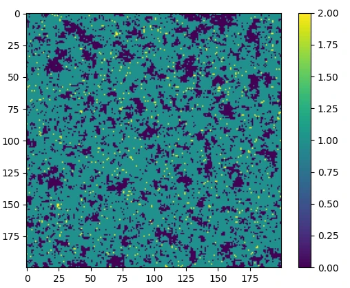
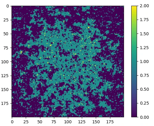
Figure 2: A sample from the Poisson-Ising model with \(\lambda=0.9\) and \(\gamma=0.8\). Left shows a sample where the Poisson rate is uniform. Right shows a sample where the Poisson rate exhibits a Gaussian decay away from the centre.

Gibbs Sampling

Sampling, in this context, is to generate random samples (or realisations) from the model. These random samples are useful for simulations, model fitting or inference. Gibbs sampling is a way to generate dependent samples by conditionally sampling each dimension of the model. In our Poisson-Ising model, this is done by sampling each pixel one at a time. Later on, we will discuss how this can be vectorised or parallelised by sampling multiple pixels at a time following some statistical properties of the model.

To initialise Gibbs sampling, we generate a random image as the starting point. Each pixel is then iteratively sampled using the CPMF. To do this, we draw a random number from a uniform distribution and use the inverse method to determine the new pixel value. Figure 3 illustrates an example of sampling a pixel. With enough iterations, the image will converge to a sample from the model.

Figure 3: An example of sampling a pixel with \(\lambda=0.9\) and \(\gamma=0.8\). The four neighbours have values 0, 2, 3, 4. Initially, this pixel has the value 1. By using the inverse method, sampling is done by changing the value of this pixel to 1 (with probability 1.7%), 2 (with probability 92.6%) or 3 (with probability 5.6%).

In terms of parallelisation, it is quite tempting to sample all pixels in parallel. However, this causes problems computationally and statistically. Statistically, only dimensions which are conditionally independent of each other can be sampled concurrently. Another way to think about it is computationally. Figure 4a) shows an example of sampling pixels adjacent to each other. Because the CPMF depends on its four neighbours, which also may change value during sampling, this can cause a data race as we read and write the same piece of data at the same time. While it is possible to tackle data races, such a sampling scheme is theoretically incorrect anyway.

Figure 4: Highlighted in blue are pixels to sample in parallel, the arrows show pixel values to be read from to sample the pixel pointed to. Left a) shows sampling pixels adjacent to each other, while right b) shows sampling pixels on a checkerboard. Arrows highlighted in red are pointing from and to blue squares, such a sampling scheme is not valid as those squares are conditionally dependent on each other and may change during sampling.

To get around this, we can concurrently sample pixels on the same colour of a checkerboard, as shown in Figure 4b). With such a sampling scheme, we can sample all pixels which are conditionally independent of each other in parallel. This makes it a good candidate for a GPU implementation as we apply the same instructions to each pixel on the checkerboard.

To ensure all pixels are sampled, we iteratively sample the pixels on the white squares on the checkerboard, followed by the black squares and so on, as illustrated in Figure 5.

Figure 5: The proposed sampling scheme. The top layer highlights in blue the pixels to sample in parallel. The bottom layer shows a checkerboard with black and white squares for illustration purposes. The left shows sampling pixels on white squares on a checkerboard, while the right is on black squares. Each iteration of Gibbs sampling will alternate between sampling white and black squares. This ensures conditionally independent pixels are sampled in parallel.

In most applications of Gibbs sampling, a user will save the sampled image after every iteration. To reduce the effects of correlation between iterations, some practitioners may use thinning, this is when samples are discarded systematically. For example, with a thinning parameter of 500, only every 500th iteration is saved as a sample, the rest are discarded.

Planning and Analysis for Software Development

With the research problem explained, it's time to discuss and plan the software development. When starting, I recommend starting with a CPU implementation or prototype. You can use it to check for correctness before you start implementing the GPU version. You would also expect both CPU and GPU implementations to give the same, or at least very similar, results. This will help you catch problems during your software development.

You can also profile and benchmark your prototype to identify bottlenecks in your CPU code. These are sections of your code where most of the CPU's time is spent on running. With the bottlenecks identified, you can focus your efforts on that particular section to speed up where it matters the most. You can use the benchmarks as a baseline to beat when you go on using multiple cores or a GPU. This is useful if, for example, you find your GPU implementation is slower. This may indicate that the technology you're using isn't suitable for your problem. Doing profiling and benchmarks during your development will hopefully steer you in the correct direction to speed up your code.

Your baseline benchmark can also be used to do a cost-benefit analysis. For example, if your prototype takes an hour to run on your full dataset, you might conclude that's good enough and that it isn't worth sending your colleagues to a GPU training course. Whilst it is technically always possible to make your code run faster, some optimisation methods may only give diminishing returns. You may also consider the training and development time, as well as monetary cost, when planning your software development to fit within a research time frame and budget. These points are important to consider to make sure your software development goes to plan.

After those considerations, I think it is important to sit down and analyse your various options and paths to speed up your code. Our docs and blog posts cover various technologies such as hybrid programming, JIT compilers and MPI. Consider the pros and cons of each before selecting one which suits your problem. This will help you make an informed choice of tools for your research problem early on in your development cycle.

CPU Implementation

We first start with discussing and commentating on the CPU implementation. A naive way would be to implement for loops to iterate for every row and column of pixels you want to sample. This is fine if you are starting off but for loops are generally slower compared to vectorising in Python. However, it is noted that the checkerboard access pattern can be tricky to implement in a vectorised form.

Suppose you have an image of size height × width. We can use np.meshgrid() to get 2D coordinates of each pixel. With that, you can work out which pixels are on black or white squares, which can be indicated by a Boolean. A code snippet is shown below

x_grid, y_grid = np.meshgrid(range(width), range(height))
checkerboard = ((x_grid + y_grid) % 2) == 0

The variable checkerboard is a matrix of Booleans with True on white squares and False on black squares. This can be used to access pixels on a checkerboard with image[checkerboard] to do Gibbs sampling. Furthermore, the variable checkerboard can be modified to switch between black and white squares after every iteration of Gibbs sampling. In addition, the matrix can be shifted by one pixel to access one of the four neighbouring pixels for calculating the interaction terms.

However, a problem occurs at the boundary. For example, if we select the top-left pixel in the image, then the neighbouring up and left pixels are out of bounds. To tackle this, we can symmetrically pad the image by one pixel using np.pad(image, 1, "symmetric"). This gives values to what would have been out-of-bound pixels. We choose symmetric padding so that the quadratic loss with the padded pixels is zero and does not contribute to the interaction terms. Figure 6 shows an illustration of this. This gives us a way to access all pixels and their neighbours, including those on the boundary, without conditionals.

Figure 6: A 3×3 image shown with solid lines. The image is symmetrically padded, indicated by numbers not surrounded by a solid line. The top-left pixel and its four neighbours are highlighted in blue. Because the top-left pixel is on the boundary, the padded pixels are highlighted too.

Putting the discussed techniques together, we can draw some pseudo-code as shown in Figure 7. Each iteration of Gibbs sampling consists of sampling the pixels on a checkerboard, alternating between black and white squares. We pad the image after each iteration to ensure the padded pixels are updated after sampling.

Figure 7: Pseudo-code and flowchart for Gibbs sampling the Poisson-Ising model. The user provides a starting image initial_image which is padded to initialise the algorithm. Each iteration of Gibbs sampling consists of sampling the pixels on a checkerboard, alternating between black and white squares after every iteration. The image is padded again after each iteration to ensure the padded pixels are updated after sampling.

With these techniques and tools, we can access data in a vectorised fashion and this is generally faster than using for loops. The vectorised format and discussed techniques can also be used as a hint or guideline when you go on implementing the GPU version, as you'll see in the next section.

GPU Implementation

When programming a GPU, you typically want to launch hundreds or thousands of threads. Naively, you can assign a thread to each pixel. However, with a checkerboard access pattern, in an iteration, half of the pixels in the image will do Gibbs sampling and the other half does nothing. Thus this assignment scheme is wasteful as it will mean half of the threads will do nothing, wasting GPU resources.

A better strategy is to assign a thread to a pair of pixels. This is illustrated in Figure 8. This way, we can make sure GPU resources are utilised well by ensuring every thread is working on a pixel which requires sampling.

Figure 8: Threads overlaid on a 4×4 image. The different colours represent different threads. The stripy shaded area represent the checkerboard pattern access, left for black squares and right for white squares. Each thread is allocated to a pair of pixels. This way, each thread will be working on a pixel on the checkerboard. This is shown as each colour, or thread, has a stripy shaded square for both figures.

One of the advantages of using CuPy is that it has many GPU implementations of NumPy functions such as cupy.pad() and cupy.random.rand(). This makes it convenient as we can choose to use these kernel functions in our GPU code rather than reimplementing them again. As a result, we can draw a similar pseudo-code, to the CPU version, as shown in Figure 9. We use cupy.random.rand() to draw random numbers from a uniform distribution. This is passed to our custom kernel gpu_sample() which samples pixels on a checkerboard using the inverse method. This alternates between white and black squares after every iteration. Lastly, like in the CPU version, we pad the image after each iteration to ensure the padded pixels are updated after sampling.

Figure 9: Pseudo-code and flowchart for Gibbs sampling the Poisson-Ising model on the GPU. The user provides a starting image initial_image which is transferred to the GPU and padded to initialise the algorithm. Each iteration of Gibbs sampling consists of drawing random numbers from a uniform distribution and using them to sample the pixels on a checkerboard, alternating between black and white after every iteration. The image is symmetrically padded afterwards. This is all done on the GPU by using cupy kernel functions and our custom kernel gpu_sample().

The pseudo-code demonstrates that CuPy helps make transferring CPU code to GPU easier by offering GPU replacements of NumPy functions. We do have to write our own custom kernel but that is the whole point of hybrid programming, to write critical parts of our code in a faster language.

It could be argued that overhead is introduced by calling multiple cupy kernel functions per iteration. An experienced programmer can reimplement cupy.pad() and cupy.random.rand() and integrate them into their custom kernel to reduce the number of kernel function calls. However, hybrid programming does enable us to be flexible and can choose what to implement in CUDA or in Python. This enables novice Python programmers to get involved with CUDA without having to use it exclusively.

When deciding what to implement in CUDA or Python, consider benchmarking and profiling to assess how much improvement can be made or where bottlenecks are. Tools such as Nsight can help you identify bottlenecks and hint where to optimise. However, do also assess readability and how it may affect accessibility and maintainability to your community. Such an assessment will help you strike a balance between languages and performance in your code.

GPU Memory Hierarchy

In this section, we will explore shared memory. This is faster, but smaller, memory allocated to each block of threads. However, with our unusual checkerboard access patterns, bank conflicts can occur which may impact performance. We will show benchmarks to investigate how different grid configurations can affect performance.

Shared memory

Threads are organised into blocks. We can provide a grid configuration by defining the block dimension and the number of blocks we want to execute in each dimension. In our problem, the block dimension consists of two numbers, the width and height of the block. We also recall VRAM, also known as global memory, is accessible by all threads. On the A100 and H100 GPUs, VRAM can be up to 80 GB.

Each block has access to its shared memory. This is smaller, but faster memory, which is only accessible by threads within a block, but not between blocks. This is illustrated in Figure 10. The size of shared memory is much smaller, the maximum size being only 48 kB per block on the A100 GPUs.

Figure 10: In this example, we allocate 8 threads per block. Each block, and thus every thread, can access global memory. Each block has access to its shared memory, which only threads within that block can access.

We can make the most of the shared memory by copying relevant data a block needs from global memory to shared memory. Threads then can exclusively work with data in shared memory without having to fetch data again from global memory. In our Gibbs sampling case, consider a block dimension of 4×2. We recall that because we allocate each thread to a pair of pixels, a block captures an 8×2 area. The relevant data to copy would be that captured area and one pixel around it too. This is so that the block can work with pixels both on black and white squares to sample, as well as the four neighbouring pixels. This is illustrated in Figure 11. This provides all the data needed by the block to work on in shared memory. Because it is in shared memory, retrieving it is faster compared to from global memory.

Figure 11: The bottom right shows the entire image (as shown by a solid grid) and a one pixel padding around it (as shown by a dashed line) which resides in global memory. The top left shows block 0, which captures the top left of the image. Highlighted blue pixels show an 8×2 area on the top left of the image and highlighted yellow shows the one-pixel padding around it . The highlighted pixels are copied to shared memory for block 0 to access and work on.

Because threads are executed concurrently in warps of 32 threads, it is advised that the number of threads per block is a multiple of 32. Selecting a good grid configuration involves experimenting, which we will demonstrate later.

Bank conflicts

The data in shared memory are stored in an array of 32 banks, each bank is 4 bytes in size which is large enough for an int or a float. Each consecutive 4 bytes of data are stored in neighbouring banks. This allows all 32 threads in a warp to retrieve data from shared memory concurrently if each thread accesses data from different banks. This will happen, for example, if your threads access adjoining data in shared memory.

A bank conflicts occur if the access pattern is unusual which causes multiple threads in a wrap to access the same bank. In a bank conflict, conflicting threads will have to access data from the same bank serially. To avoid this, we can select a block dimension which prevents this. For illustration purposes, we show an example with 12 banks and a block dimension of 6×2 in Figure 12. In this example, the top row selects odd indices and the bottom row even indices due to our block dimension, the checkerboard access pattern and the one pixel padding. This guarantees that each thread accesses a unique bank.

Figure 12: a) The contents of shared memory with a block dimension of 6×2. The solid lines show the image covered by the block. Each pixel is labelled by an index sequentially. Highlighted in blue is the checkerboard access pattern. b) How the data in shared memory are arranged in banks. In this example, we have 12 banks. There are no bank conflicts as each thread is accessing different banks.

Figure 13 shows another example with a block dimension of 2×6, where such a block dimension causes a 4-way bank conflict.

Figure 13: a) The contents of shared memory with a block dimension of 2×6. The solid lines show the image covered by the block. Each pixel is labelled by an index sequentially. Highlighted in blue is the checkerboard access pattern. b) How the data in shared memory are arranged in banks. In this example, we have 12 banks. With a checkerboard access pattern, the 12 threads cause a 4-way bank conflict as we have more than one thread accessing the same bank.

One way to avoid bank conflicts is to pad the shared memory with unused data. Continuing with our block dimension of 2×6, Figure 14 shows an example of padding the shared memory by two pixels. By adding a padding, it avoids bank conflicts by shifting the indices on each row by two, which in turn shifts which bank is accessed by each thread. We choose a padding size so that each thread accesses a unique bank.

However, this technique will not work on skinny block dimensions such as 12×1.

Figure 14: a) The contents of shared memory with a block dimension of 2×6 with an additional 2 pixels of padding to the right. The solid lines show the image covered by the block. Each pixel is labelled by an index sequentially. Highlighted in blue is the checkerboard access pattern. b) How the data in shared memory are arranged in banks. In this example, we have 12 banks. With a checkerboard access pattern and the extra padding, the 12 threads can all access a different bank.

It is given that for 32 banks and 32 threads in a block, the following grid configurations produce no bank conflicts

• 16×2
• 8×4 + 6
• 4×8 + 2
• 2×16

where, for example, 8×4 + 6 means a block dimension of 8×4 with a 6 pixel padding. For more than 32 threads in a block, the heights in the above block dimensions can be multiplied by an integer amount, for example, 16×4 and 8×8 + 6.

Benchmarks

We did a benchmark using various grid configurations to investigate how different grid configurations affected performance. We used the Python package pytest-benchmark to re-use some of my test code and to parameterise the grid configuration.

In our benchmarks, we obtained 1000 samples of a 2048×2048 image, with a thinning parameter of 500. We used a Poisson rate of \(\lambda=0.9\) which exhibits a Gaussian decay away from the centre, that is

\[ \lambda_{i,j}= 0.9 \times \exp\left[ -\left(\dfrac{i-1028}{3427}\right)^2 -\left(\dfrac{j-1028}{3427}\right)^2 \right] \]

We also used an interaction coefficient of \(\gamma=0.8\). The benchmarks are repeated 32 times to see how the timing varies.

A summary of the timings is shown in Figure 15 as a bar chart. The exact timings in a table with their corresponding grid configurations are shown in Figure 19 in the appendix.

Figure 15: Benchmarks on the V100, A100 and H100 GPUs. For a given GPU, the different bars correspond to different grid configurations, as shown in the table in Figure 19. The bars are ordered from fastest to slowest.

The biggest effect on the benchmarks is the model of GPU used, with the newer GPUs consistently outperforming the older ones. The next biggest factor is the block dimensions. We found that, for a given GPU, fiddling about with the block dimension can gain you up to between 50-70% performance gain. In some cases, bad grid configurations will degrade benchmarks to the point they perform similarly to an older GPU. However, towards the optimal end, we've found that the top 10 to 15 grid configurations give practically similar benchmarks to each other.

For block dimensions with widths 4 and 8, adding padding to shared memory will prevent bank conflicts. We have found statistical evidence of improvement in benchmarks when doing this. In Figure 16, we compared those grid configurations with and without padding and found that adding padding consistently and statistically improves performance. Practically, however, this improvement is negligible, in the order of fractions of seconds.

Figure 16: Bland-Altman difference plot comparing the benchmarks of grid configurations with and without padding in shared memory. Each point represents a grid configurations and each colour for a different GPU model. Only block dimensions with widths 4 and 8 are considered. The x-axis shows the average of the two benchmarks and the y-axis the difference. The error bars show the combined standard deviation from the 32 repeats. The dashed line is at zero and negative values underneath that line show that adding padding improves benchmarks.

The main driving factors for choosing a good grid configuration are the number of warps per block and the width of the block. Figure 17 shows the A100 benchmarks with different grid configurations organised into different numbers of warps per block. Going from one warp per block to two shows about a 10% improvement, but any more shows no noticeable difference. The improvement arises because blocks are assigned to streaming multiprocessors (SMs) and having multiple warps per block ensures that SMs have enough active threads to hide latency and fully utilise GPU resources.

Figure 17: Benchmarks from the A100 GPU. Each bar represents a grid configuration, with shared memory padding where applicable, and are organised into number of warps per block. Only the top 5 from each number of warps per block are shown and are ordered from fastest to slowest.

Next, Figure 18 shows the benchmarks organised into the widths of the block. It can be seen that having a block width of one is detrimental to performance but improves up to a block width of 4. For this particular problem, we suggest a block width of at least 4. Bank conflicts, by themselves, aren't the cause of this. As discussed before, padding the shared memory to avoid bank conflicts gives negligible improvements. We've also observed block widths of 32, and even 64 and beyond, still give respectable results.

The one outlier we see for block widths 4, 8, 16 and 32, is due to including benchmarks with only one warp per block, which, as discussed before, also destroys performance.

Figure 18: Benchmarks from the A100 GPU. Each bar represents a grid configuration and is organised into the width of the block. Block heights of 32, 64, 128 and 256 are shown, and where applicable, with shared memory padding. For each block width, the benchmarks are ordered from fastest to slowest. Block widths of 2, 4, 8 and 16 should have no bank conflicts.

In summary, our benchmarks have led to some useful rules of thumb for choosing grid configurations. While certain configurations, such as a block width of one, perform disastrously, once a good configuration is found, the choice becomes less critical, as many reasonable configurations yield similarly optimal performance.

Conclusion

CuPy is a great tool for hybrid Python and CUDA programming, utilising both languages to our advantage. We also found that CuPy's reimplementation of NumPy functions could help novice GPU programmers transition their CPU code to the GPU. With familiar functions in our code, it will also make the code accessible to Python programmers should the code be maintained in the future.

When studying the Gibbs sampler for the Poisson-Ising model, the unusual checkerboard access pattern along with the symmetric padding meant that assigning threads to data was a bit more involved. We assigned pairs of pixels to a thread to ensure each thread was working and utilised well. We also looked at using faster shared memory and how to prevent bank conflicts.

We've observed that newer and faster GPUs give better performance and are the main significant factor in our benchmarks. For a given GPU, performance can be improved by tuning the grid configuration, albeit relatively modestly. In some cases, up to a 50-70% performance gain can be achieved by fiddling around with the block dimension. We advise trying out different grid configurations to find ones which perform well before using them in a full run. But once a good enough grid configuration is found, further fine-tuning gives negligible improvements.

Hopefully, with these tools and advanced concepts, a Python programmer can have a go programming in CUDA without having to completely leaving the Python ecosystem. This will help make GPUs accessible to academics and researchers with various expertise in programming.

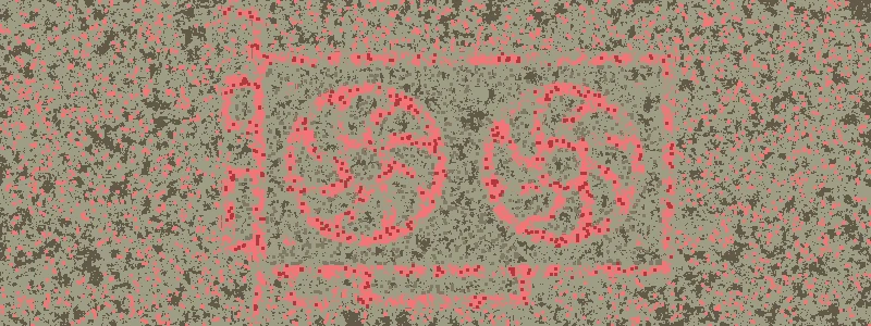
About the header image

I've used an icon of a GPU as the Poisson rate to do Gibbs sampling. The colours were chosen to be difficult to see with red colour-blindness or if you print it in black and white. This is a play on the Ishihara test.

Appendix

V100 on sbg		A100 on rdg		H100 on xdg
Grid config.	Time (s)	Grid config.	Time (s)	Grid config.	Time (s)
128×1	177.71±0.06	32×2	93.26±0.06	32×4	69.310±0.026
64×2	177.913±0.027	16×8	93.29±0.06	64×2	69.313±0.017
128×2	177.918±0.011	64×2	93.2962±0.0029	32×2	69.326±0.024
64×4	178.374±0.007	32×4	93.302±0.004	16×4	69.374±0.029
32×4	178.42±0.04	16×4	93.32±0.07	64×4	69.378±0.008
32×2	178.44±0.04	128×2	93.43±0.06	128×2	69.379±0.011
64×1	178.570±0.035	64×4	93.44±0.06	16×8	69.387±0.025
32×8	178.950±0.015	64×1	93.49±0.06	64×1	69.389±0.017
256×1	179.049±0.032	32×8	93.50±0.06	128×1	69.400±0.012
16×8	179.660±0.014	8×16 + 6	93.52±0.08	32×8	69.417±0.015
16×4	179.777±0.018	128×1	93.5273±0.0030	256×1	69.521±0.015
16×16	180.94±0.05	16×16	93.55±0.06	8×8 + 6	69.607±0.035
8×8 + 6	181.04±0.11	8×8 + 6	93.68±0.05	16×16	69.63±0.05
8×16 + 6	181.68±0.11	8×16	93.69±0.06	8×8	69.681±0.035
8×8	181.94±0.10	8×32 + 6	93.79±0.05	8×16 + 6	69.68±0.04
8×16	182.62±0.11	256×1	93.79±0.07	8×16	69.766±0.030
8×32 + 6	183.56±0.07	8×8	93.93±0.04	8×32 + 6	69.853±0.022
8×32	184.43±0.06	8×32	94.11±0.06	8×32	69.935±0.025
4×16 + 2	185.83±0.13	4×16 + 2	95.303±0.005	4×16 + 2	70.856±0.025
4×16	187.29±0.12	4×32 + 2	95.478±0.010	4×32 + 2	70.988±0.019
4×32 + 2	189.424±0.011	4×64 + 2	96.192±0.008	4×16	71.180±0.021
32×1	190.09±0.10	4×16	96.746±0.008	4×32	71.248±0.016
4×32	190.87±0.05	4×32	97.11±0.04	4×64 + 2	71.258±0.015
8×4 + 6	191.51±0.05	4×64	97.69±0.06	4×64	71.557±0.010
16×2	191.772±0.011	32×1	102.654±0.005	32×1	72.674±0.022
4×8 + 2	191.884±0.035	16×2	102.67±0.07	16×2	73.067±0.026
8×4	192.20±0.07	2×64	103.00±0.06	8×4 + 6	73.515±0.034
4×64 + 2	192.34±0.07	8×4 + 6	103.296±0.010	8×4	73.646±0.017
4×8	192.89±0.06	2×32	103.330±0.034	4×8 + 2	74.672±0.028
4×64	193.58±0.07	8×4	103.823±0.009	4×8	74.981±0.030
2×16	199.990±0.032	2×128	104.182±0.031	2×32	75.268±0.015
2×128	212.35±0.06	4×8 + 2	104.498±0.016	2×64	75.460±0.033
2×32	212.78±0.15	4×8	105.37±0.09	2×128	75.744±0.022
2×64	217.35±0.04	2×16	108.359±0.029	2×16	77.828±0.035
1×32	249.00±0.14	1×128	139.572±0.029	1×64	94.574±0.034
1×256	273.85±0.04	1×256	139.742±0.006	1×128	95.704±0.032
1×64	273.911±0.023	1×32	141.34±0.22	1×32	95.95±0.12
1×128	274.324±0.030	1×64	142.906±0.031	1×256	96.28±0.05

Figure 19: Table of benchmarks on the V100, A100 and H100 GPUs. Quoted are the mean and standard deviations. Different grid configurations were used, for example, 8×4 + 6 means a block dimension of 8×4 with a 6 pixel padding on the shared memory.